Panorama Stitching

Setting

If the camera center is fixed, or if the scene is planar, different images of the same scene are related by a homography. In this project, you will implement an algorithm to calculate the homography between two images. Several images of each scene will be provided. Your program should generate image mosaics according to these estimated homographies.

To accomplish panorama stitching, the following pipeline is commonly used:

1. Feature detection.
2. Feature matching.
3. Homography estimation.
4. Panorama stitching.

The data given has four folders, each including 3-6 photos on different perspectives. Note that the sequence of the photos are not concerned to the actual shooting angle.

Environment

• OS: Windows 11 24H2
• Lib: Python 2.7, Opencv 3.4.2.16

Algorithm

1. The Basic Algorithm

1.1 Feature Detection, Descriptor, and Matching

The first step in panorama stitching is identifying common features between pairs of images. These features allow us to align the images correctly. The code uses the Matchers class to perform this step, which utilizes the SURF (Speeded-Up Robust Features) algorithm and FLANN-based matching.

Feature Detection and Descriptor Computation:

• SURF is used to detect distinctive keypoints in each image and compute descriptors. Keypoints are regions in the image that are easily identifiable and remain consistent across different views of the scene (such as corners, edges, or blobs). The descriptors are mathematical representations of the keypoints that allow for comparison between images.

  In the Matchers class, the method _get_features(image):

  keypoints, descriptors = self.surf.detectAndCompute(gray, None)

  converts the image to grayscale, detects keypoints, and computes the descriptors for matching.

Matching Keypoints:

Once the descriptors are extracted, the match method in the Matchers class uses the FLANN (Fast Library for Approximate Nearest Neighbors) matcher to find the best matches between keypoints from two images:

matches = self.flann.knnMatch(features2['des'], features1['des'], k=2)

For each keypoint in image2, the two closest matches are found in image1. The code then applies the ratio test (Lowe’s ratio test) to filter out poor matches. Only good matches are retained for the homography calculation:

good_matches.append((m.trainIdx, m.queryIdx))

1.2 Homography Estimation

Once keypoints are matched, the next step is to estimate the homography matrix, which represents the transformation required to align the two images. This transformation is essential to align the images in the panorama seamlessly.

Homography Calculation:

The match method uses the RANSAC algorithm (Random Sample Consensus) to calculate the homography matrix. RANSAC helps to eliminate outliers, ensuring that only reliable matches are used to compute the transformation.

• The keypoints of the matching pairs are converted into float32 coordinates:

  points1 = np.float32([features1['kp'][i].pt for (i, _) in good_matches])
  points2 = np.float32([features2['kp'][i].pt for (_, i) in good_matches])

• Then, the findHomography function calculates the homography matrix H:

  H, _ = cv2.findHomography(points2, points1, cv2.RANSAC, 4)

  The result is the homography matrix H, which defines how to warp one image to align with the other.

Homography Score:

The quality of the homography matrix can be assessed by calculating its norm using the _calculate_homography_score(H) method:

return np.linalg.norm(H)

A lower norm indicates a better match.

1.3 Image Stitching

With the homography matrices in hand, the next step is to stitch the images together to form the final panorama.

Image Alignment:

The Stitcher class has two main methods to handle the alignment process: _shift_left and _shift_right.

• Left-side Image Alignment (_shift_left):

  • Starting from the center image, images on the left are aligned one by one by applying their respective homography matrices. The transformation is applied using cv2.warpPerspective, which warps the image based on the homography matrix H.

  • The code ensures that the resulting image has enough space to accommodate the newly aligned image by adjusting the size dynamically.

  • Images are gradually merged using pixel-wise blending to avoid seams.

    tmp = cv2.warpPerspective(a, xh, dsize)

• Right-side Image Alignment (_shift_right):

  • Similarly, images on the right are aligned and stitched into the panorama. The right images are warped and blended into the final stitched image.

Blending Images:

To avoid visible seams between adjacent images, the _blend_images method is used to combine the images smoothly. It creates a weighted average of pixel values at overlapping regions:

blended_image[y, x] = (
    blended_image[y, x].astype(np.float32) * 0.5 +
    warped_image[y, x].astype(np.float32) * 0.5
).astype(np.uint8)

This ensures that the final panorama looks seamless, with no visible boundaries between the images.

Final Panorama Creation:

Once all images are aligned and blended, the final panorama is created, starting from the center image and progressively stitching images on the left and right. The stitch() method returns the final stitched image:

return self.left_image

2. Comparison of different feature descriptors

Descriptor Extraction:

• SIFT: Extracts scale-invariant keypoints and computes descriptors based on local image gradients (sift_descriptor function).
• Pixel-based: Detects keypoints using corner detection and creates descriptors from pixel values in local patches (pixel_descriptor function).

Descriptor Matching: The match_descriptors function uses FLANN-based matching to find potential matches between the descriptors of the two images.

Homography Estimation with RANSAC: The estimate_homography function uses RANSAC to estimate a transformation between the images and counts inliers (correct matches). RANSAC is run multiple times, and the best transformation is chosen based on the number of inliers.

RANSAC Iterations Calculation: The calculate_ransac_iterations function computes how many iterations are needed to achieve a specified success probability based on the inlier ratio.

Performance Evaluation: The compare_descriptors function compares the two descriptors by calculating the inlier ratio and required RANSAC iterations. It visualizes matches and evaluates the descriptors' performance using RANSAC on a set of random matches.

Experiments

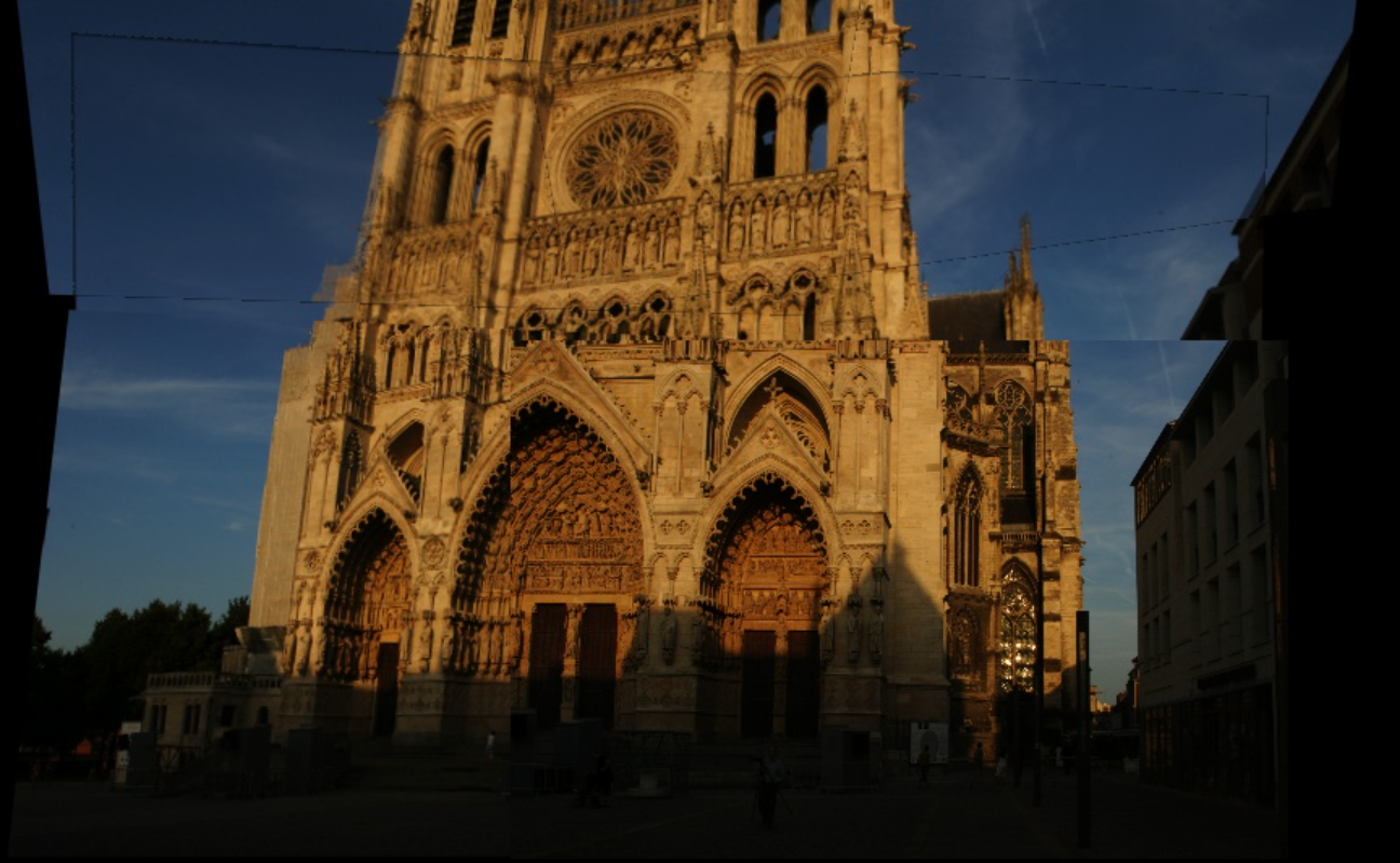
1. Image Stitching

dataset	result
data1
data2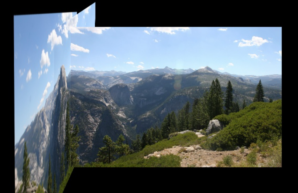
data3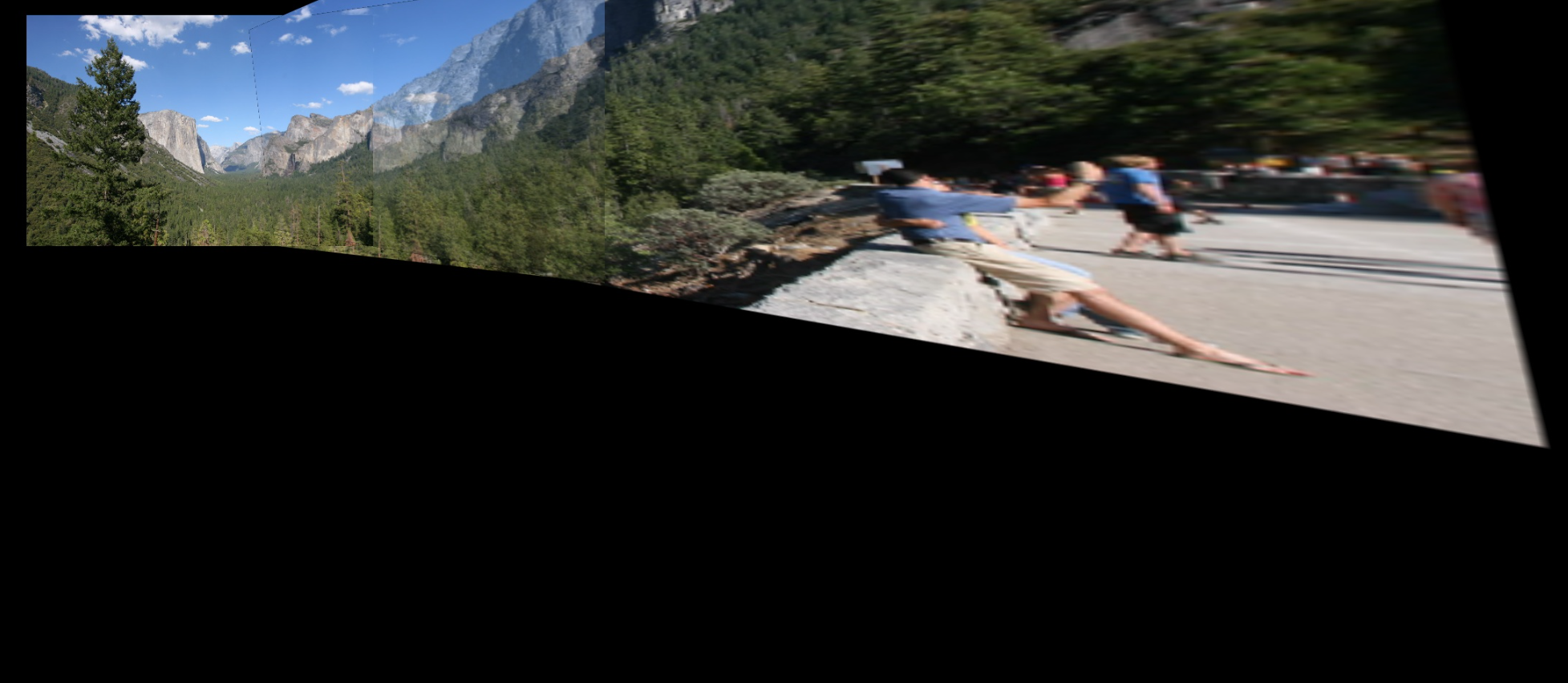
data4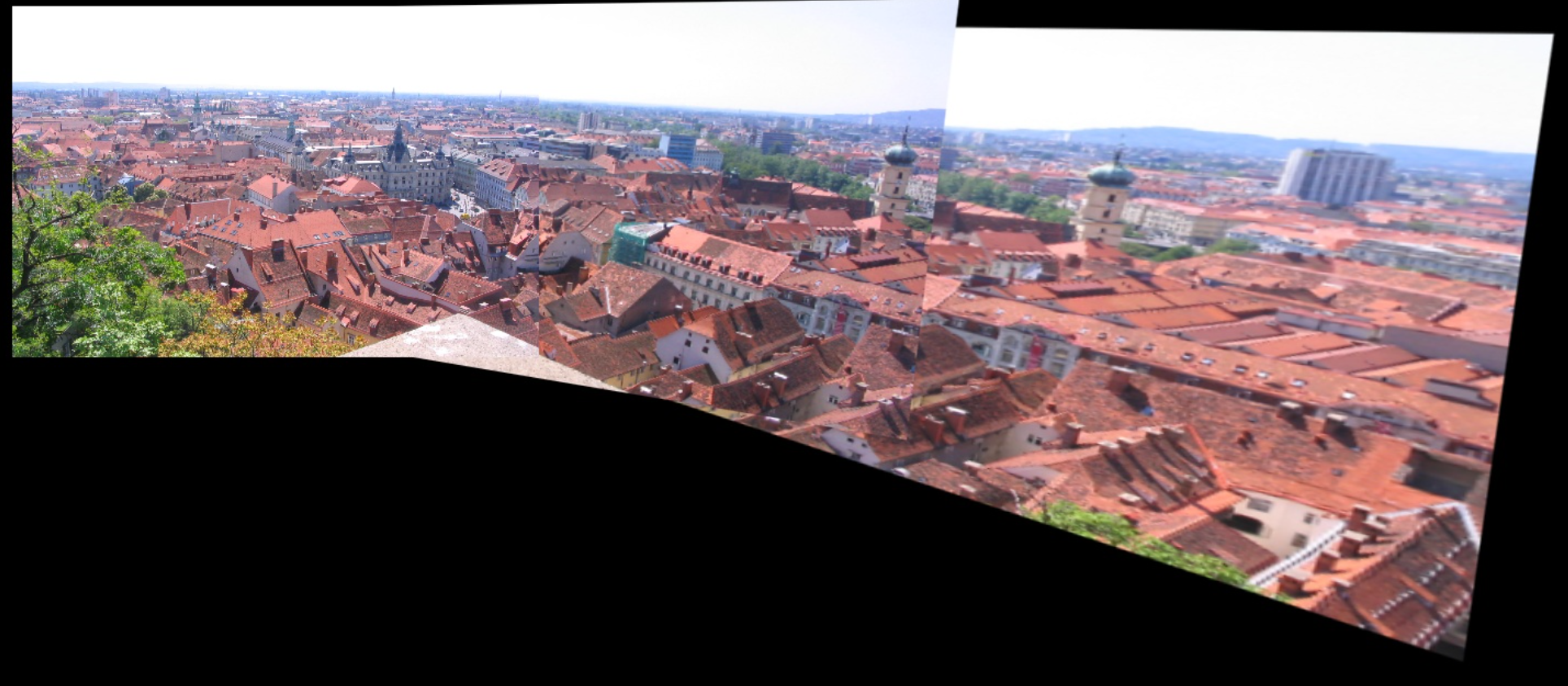

Though my algorithm accomplishes panorama stitching, there is obviously a way to improve. My result shows that the stitchings are starting with the picture on the edge, but it's proper to start from the middle. Though I've set the picture which has the most matching with other pics as the base picture, it turns out to be the the most marginal one. It's confusing. Anyway, the result is sufficent, at least a lot better than the code I first wrote.

2. Comparison of feature descriptors

This is a matching result (taking data4/IMG_7357.JPG and data4/IMG_7358.JPG as example):

descriptor	matching result
SIFT
Pixel

This is the summarizing table:

dataset	iteration (SIFT)	iteration (Pixel)	average ratio (SIFT)	average ratio (Pixel)
data1/112_1298.JPG data1/112_1299.JPG	24	26	0.41	0.40
data2/IMG_0488.JPG data2/IMG_0489.JPG	22	26	0.42	0.40
data3/IMG_0675 data3/IMG_0676	25	25	0.40	0.40
data4/IMG_7357 data4/IMG_7358	23	26	0.41	0.40

It shows that SIFT descriptor contributes to less iterations and better average inlier ratio.